Soil Correlations and Approximations Employed in this Study

Automating capacity calculations posed several challenges. When either performing hand calculations or using standard commercial software applications, the geotechnical engineer is responsible for preparing the load test record for analysis by reducing boring logs, lab test results and other relevant data to a generalized soil profile with average geotechnical properties per layer. Moving from a one-at-a-time analysis to batch processing hundreds of load test records required writing algorithms that could reliably substitute a lot of the engineer’s manual pre-processing.

All the algorithms were eventually compiled in an installable Python module called edafos. The source code is available at https://github.com/nickmachairas/edafos. Being open source, this project can be adopted and extended by interested users confortable with Python programming. Being modular, this project can be used to support other applications. edafos is running all geotechnical analysis and capacity calculations for the NYU Pile Capacity web application presented in Chapter 2.

A key issue with the available load test records is missing values of geotechnical properties. And while it might seem too simple, soil property approximations were crucial in calculating in-situ stresses and pile capacities.

Correlations

Olson

Most of the values of total unit weight (TUW, a.k.a. moist unit weight), \(\gamma_t\), in Prof. Roy Olson’s database were assumed. If water content, \(w\), was known, it was used to calculate \(\gamma_t\), with an assumed specific gravity, \(G_s\), of 2.72. In this case, \(\gamma_t\) is given by Eq. 1.

(1)\[\gamma_t = \bigg( \dfrac{1 + w}{1 + w G_s} \bigg) \; G_s \gamma_w\]

Prof. Olson used cases in which water contents were measured to calculate total unit weights for all soils and then performed correlations of those values of total unit weight with whatever other properties were available, meaning undrained shear strength, \(s_u\), for cohesive soils, and SPT-N values for all soils, and used these other properties to estimate total unit weight for cases in which water contents were not defined. These correlations were often poor but they gave a consistent basis for estimating \(\gamma_t\). The correlations are shown below for cohesive and cohesionless soils.

Cohesive Soils

Values for undrained shear strength may come from the following:

• Field vane shearing strength (\(s_{u.FV}\))

• Shearing strength from Torvane, penetrometer, etc (\(s_{u.MS}\))

• Shearing strength from triaxial tests (\(s_{u.QT}\))

• Unconfined shearing strength (\(s_{u.UU}\))

Priority for choosing a value for \(s_u\) if multiple are available is:

\[s_{u.QT} > s_{u.UU} > s_{u.MS} > s_{u.FV}\]

But must adjust according to Eq. 2:

(2)\[\begin{split}s_u = \begin{cases} s_{u.QT} \\ 1.2 \times s_{u.UU} \\ 1.2 \times s_{u.MS} \\ 0.7 \times s_{u.FV} \end{cases}\end{split}\]

Correlations were adjusted depending on the specific type of the cohesive soil. Different equations were produced for clays (CLAY) and silty clays (SICL), clayey silts (CLSI) and sandy clays (SACL). All cases are summarized in Eq. 3 and Eq. 4. \(s_u\) must be provided in ksf and \(\gamma_t\) is returned in pcf.

Note

If both SS and N were undefined, TUW was set to 0 as code that values of EVSO cannot be defined.

For clay (CLAY):

(3)\[\begin{split}\gamma_t = \begin{cases} 113.9 + 9.276 \ln{s_u} \textrm{ in pcf} & \textrm{if } s_u > 0 \textrm{ in ksf} \\ 107.5 + 5.116 \ln{N} \textrm{ in pcf} & \textrm{if } s_u \textrm{ undef. and } N > 0 \\ \textrm{N/A} & \textrm{if both } s_u \textrm{ and } N \textrm{ are undefined} \end{cases}\end{split}\]

For silt/clay (SICL), clay/silt (CLSI) and sand/clay (SACL):

(4)\[\begin{split}\gamma_t = \begin{cases} 113 + 22 s_u \textrm{ in pcf} & \textrm{if } 0.5 < s_u < 1.5 \textrm{ in ksf} \\ 113 + 9.276 \ln{N} \textrm{ in pcf} & \textrm{if } s_u > 0 \\ \textrm{N/A} & \textrm{if both } s_u \textrm{ and } N \textrm{ are undefined} \end{cases}\end{split}\]

Cohesionless Soils

Correlations for cohesionless soils depended on the soil type. Eq. 5 summarises cases for sands (SAND), silty sands (SISA), sandy silts (SASI), silts (SILT), cobbles/gravels (CBGV), gravels (GRAV), sandy gravels (SAGV), gravely sands (GVSA), cobbles (COBB).

(5)\[\begin{split}\gamma_t = \begin{cases} 126 \textrm{ pcf} & \textrm{for} \quad \textrm{SAND} \\ 125 + 0.15 N < 135 \textrm{ pcf} & \textrm{for} \quad \textrm{SISA, SASI, SILT} \\ 132 \textrm{ pcf} & \textrm{for} \quad \textrm{CBGV, GRAV, SAGV, GVSA, COBB} \end{cases}\end{split}\]

Olson Soil Classification to USCS

Table 1 Appendix: Olson Soil Classification to Unified Soil Classification System (USCS)

Olson				USCS
Symbol	Description	Category	Count 1	Symbol	Description
CLAY	Clay	Cohesive	2305	CL	Inorganic clays of low to medium plasticity, gravelly clays, sandy clays, silty clays, lean clays
CLSA	Clay/Sand	Cohesive	3	SC	Clayey sands, sand-clay mixtures
CLSI	Clay/Silt	Cohesive	20	ML	Inorganic silts, and very fine sands, rock flour, silty or clayey fine sands or clayey silts with slight plasticity
GRAV	Gravel	Coarse	49	GW or GP	Well/Poorly-graded gravels, gravel-sand mixtures, little or no fines
GVSA	Gravel/Sand	Coarse	45	GW or GP	Well/Poorly-graded gravels, gravel-sand mixtures, little or no fines
MISA	Micaceous Sand	Cohesionless	15	MH	Inorganic silts, micaceous or diatomaceous fine sandy or silty soils, elastic silts
MISS	Micaceous Sand/Silt	Cohesionless	6	MH	Inorganic silts, micaceous or diatomaceous fine sandy or silty soils, elastic silts
PEAT	Peat	Cohesive	1	PT	Peat and other highly organic soils
SACL	Sand/Clay	Cohesive	14	SC	Clayey sands, sand-clay mixtures
SAGV	Sand/Gravel	Coarse	67	GW or GP	Well/Poorly-graded gravels, gravel-sand mixtures, little or no fines
SAND	Sand	Cohesionless	1780	SW or SP	Well/Poorly-graded sands, gravelly sands, little or no fines
SASI	Sand/Silt	Cohesionless	319	SM	Silty sands, sand-silt mixtures
SHEL		Coarse	2	GW or GP	Well/Poorly-graded gravels, gravel-sand mixtures, little or no fines
SICL	Silt/Clay	Cohesive	39	ML	Inorganic silts, and very fine sands, rock flour, silty or clayey fine sands or clayey silts with slight plasticity
SILT	Silt	Cohesionless	198	MH	Inorganic silts, micaceous or diatomaceous fine sandy or silty soils, elastic silts
SISA	Silt/Sand	Cohesionless	397	SM	Silty sands, sand-silt mixtures

Hunt

Roy Hunt on his 1984 book, the “Geotechnical Engineering Investigation Manual” (Hunt, 1984), offers typical values for common properties including relative density, \(D_r\), dry density, \(\gamma_{dry}\), void ratio, \(e\), and strength, \(\phi\), as related to gradation and SPT-N. For cohesionless soils these typical values are presented in Table 2.

For cohesive soils, common properties, including relationships between consistency, unconfined compressive strength, \(q_u\), saturated weight, \(\gamma_{sat}\), and SPT-N are given on Table 3. Furthermore, typical properties of cohesive materials classified by geologic origin, including density, \(\gamma_{dry}\), natural moisture contents, \(w\), plasticity indices, \(PI\) and strength parameters, \(s_u, c, \phi\), are given on Table 4.

Table 2 Appendix: Common Properties of Cohesionless Soils (after Hunt, 1984)

Material	Compactness	\(D_r\), %	N 2	\(\gamma_{dry}\) 3, lbf/ft3	Void Ratio, \(e\)	Strength 4, \(\phi\)
GW: well-graded gravels, gravel- sand mixtures	Dense	75	90	138	0.22	40
	Medium dense	50	55	130	0.28	36
	Loose	25	< 28	123	0.36	32
GP: poorly graded gravels, gravel- sand mixtures	Dense	75	70	127	0.33	38
	Medium dense	50	50	120	0.39	35
	Loose	25	< 20	114	0.47	32
SW: well-graded sands, gravelly sands	Dense	75	65	118	0.43	37
	Medium dense	50	35	112	0.49	34
	Loose	25	< 15	106	0.57	30
SP: poorly graded sands, gravelly sands	Dense	75	50	110	0.52	36
	Medium dense	50	30	104	0.60	33
	Loose	25	< 10	99	0.65	29
SM: silty sands	Dense	75	45	103	0.62	35
	Medium dense	50	25	97	0.74	32
	Loose	25	< 8	93	0.80	29
ML: inorganic silts, very fine sands	Dense	75	35	93	0.80	33
	Medium dense	50	20	88	0.90	31
	Loose	25	< 4	84	1.00	27

Table 3 Appendix: Common Properties of Cohesive Soils (after Hunt, 1984)

Consistency	N	Hand test	\(\gamma_{sat}\) 5, lbf/ft3	Strength 6, \(q_u\), kip/ft2
Hard	> 30	Difficult to indent	> 140	> 8.2
Very stiff	15 - 30	Indented by thumbnail	130 - 140	4.1 - 8.2
Stiff	8 - 15	Indented by thumb	120 - 130	2.0 - 4.1
Medium (firm)	4 - 8	Molded by strong pressure	110 - 120	1.0 - 2.0
Soft	2 - 4	Molded by slight pressure	100 - 110	0.5 - 1.0
Very soft	< 2	Extrudes between fingers	90 - 100	0.0 - 0.5

Table 4 Appendix: Typical Properties of Formations of Cohesive Materials (after Hunt, 1984)

Material	Type	Location	\(\gamma_{dry}\), lbf/ft3	\(w\), %	LI, %	PI, %	\(s_u\), kip/ft2	\(\bar{c}\), kip/ft2	\(\bar{\phi}\)	Remarks
CLAY SHALES (WEATHERED)
Carlisle (Cret.)	CH	Nebraska	92	18				1.024	45	\(\phi\) extremely variable
Bearpaw (Cret.)	CH	Montana	90	32	130	90		0.717	15
Pierre (Cret.)	CH	South Dakota	92	28				1.843	12
Cucaracha (Cret.)	CH	Panama Canal		12	80	45				\(\phi_r = 10^\circ\)
Pepper (Cret.)	CH	Waco, Texas		17	80	58		0.819	17	\(\phi_r = 7^\circ\)
Bear Paw (Cret.)	CH	Saskatchewan		32	115	92		0.819	20	\(\phi_r = 8^\circ\)
Modelo (Tert.)	CH	Los Angeles	90	29	66	31		3.277	22	Intact specimen
Modelo (Tert.)	CH	Los Angeles	90	29	66	31		0.655	27	Shear zone
Martinez (Tert.)	CH	Los Angeles	104	22	62	38		0.512	26	Shear zone
(Eocene)	CH	Menlo Park, Calif.	103	30	60	50		Free swell 100%; P = 20.5 kip/ft2
RESIDUAL SOILS
Gneiss	CL	Brazil; buried	81	38	40	16		0.000	40	\(e_0 = 1.23\)
Gneiss	ML	Brazil; slopes	84	22	40	8		0.799	19	\(c, \phi\): unsoaked
Gneiss	ML	Brazil; slopes	84		40	8		0.573	21
COLLUVIUM
From shales	CL	West Virginia		28	48	25		0.573	28	\(\phi_r = 16^\circ\)
From gneiss	CL	Brazil	69	26	40	16		0.410	31	\(\phi_r = 12^\circ\)
ALLUVIUM
Black swamp	OH	Louisiana	36	140	120	85	0.307
Black swamp	OH	Louisiana	62	60	85	50	0.205
Black swamp	MH	Georgia	60	54	61	22	0.614			\(e_0 = 1.7\)
Lacustrine	CL	Great Salt Lake	49	50	45	20	0.696
Lacustrine	CL	Canada	69	62	33	15	0.512
Lacustrine (volcanic)	CH	Mexico City	18	300	410	260	0.819			\(e_0 = 7\), \(S_t = 13\)
Estuarine	CH	Thames River	49	90	115	85	0.307
Estuarine	CH	Lake Maricaibo		65	73	50	0.512
Estuarine	CH	Bangkok		130	118	75	0.102
Estuarine	MH	Maine		80	60	30	0.410
MARINE SOILS (OTHER THAN ESTUARINE)
Offshore	MH	Santa Barbara, Calif.	52	80	83	44	0.307			\(e_0 = 2.28\)
Offshore	CH	New Jersey		65	95	60	1.331
Offshore	CH	San Diego	36	125	111	64	0.205			Depth = 6.56 ft
Offshore	CH	Gulf of Maine	36	163	124	78	0.102
Coastal Plain	CH	Texas (Beaumont)	87	29	81	55	2.048	0.410	16	\(\phi_r = 14^\circ\), \(e_0 = 0.8\)
Coastal Plain	CH	London	100	25	80	55	4.096
LOESS
Silty	ML	Nebraska-Kansas	77	9	30	8		1.229	32	Natural \(w\) %
Silty	ML	Nebraska-Kansas	77		30	8		0.000	23	Prewetted
Clayey	CL	Nebraska-Kansas	78	9	37	17		4.096	30	Natural \(w\) %
GLACIAL SOILS
Till	CL	Chicago	132	23	37	21	7.169
Lacustrine (varved)	CL	Chicago	106	22	30	15	2.048			\(e_0 = 0.6\) (OC)
Lacustrine (varved)	CL	Chicago		24	30	13	0.205			\(e_0 = 1.2\) (NC)
Lacustrine (varved)	CH	Chicago	74	50	54	30	0.205
Lacustrine (varved)	CH	Ohio	60	46	58	31	1.229			\(S_t = 4\)
Lacustrine (varved)	CH	Detroit	75	46	55	30	1.639			\(e_0 = 1.3\) (clay)
Lacustrine (varved)	CH	New York City		46	62	34	2.048			\(e_0 = 1.25\) (clay)
Lacustrine (varved)	CL	Boston	84	38	50	26	1.639			\(S_t = 3\)
Lacustrine (varved)	CH	Seattle		30	55	22			30	\(\phi_r = 13^\circ\)
Marine 7	CH	Canada-Leda clay	56	80	60	32	1.024			\(S_t = 128\)
Marine 7	CL	Norway	84	40	38	15	0.266			\(S_t = 7\)
Marine 7	CL	Norway	81	43	28	15	0.102			\(S_t = 75\)

1

Count in Olson ‘APC’ and ‘CT’ databases.

2

\(N\) is blows per foot of penetration in the SPT. Adjustments for gradation are after Burmister (1962).

3

Density given is for \(G_s = 2.65\) (quartz grains)

4

Friction angle \(\phi\) depends on mineral type, normal stress, and grain angularity as well as \(D_r\) and gradation.

5

\(\gamma_{sat} = \gamma_{dry} + \gamma_w \Big( \dfrac{e}{1+e} \Big)\)

6

Unconfined compressive strength, \(q_u\), is usually taken as equal to twice the cohesion, \(c\), or the undrained shear strength, \(s_u\). For the drained strength condition, most clays also have the additional strength parameter, \(\phi\), although for most normally consolidated clays, \(c = 0\). Typical values for \(s_u\) and drained strength parameters are given in Table 4.

7(1,2,3)

Marine clays strongly leached.

Layer Delineation

Most of the design problems encountered in Soil Mechanics involve calculations with geotechnical properties of soil profiles that have been deduced from raw geotechnical data. Case in point, recommended step-by-step design procedures within the 2006 version of the FHWA Driven Pile Foundation Manual (Hannigan et al., 2006a) start by delineating the soil profile into layers using soil test data.

The process of delineating the soil profile into layers is easier said than done and is based on engineering judgement and experience. Fig. 1 shows the SPT N values collected during field tests for “North Abutment S-1” (after Hannigan et al., 2006a).

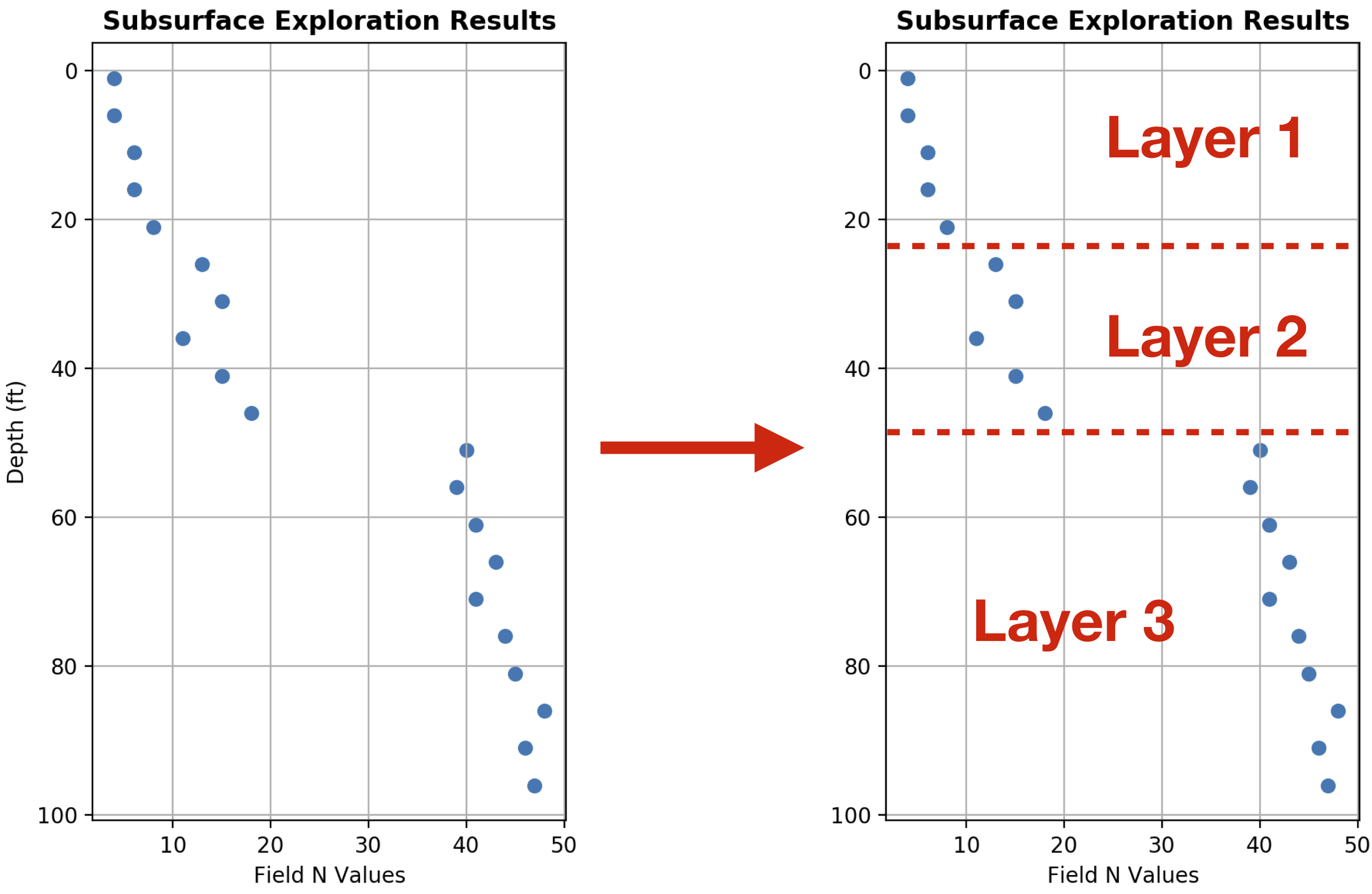
Fig. 1 Appendix: Delineating the soil profile into layers using the field SPT N Values for “North Abutment S-1” (after Hannigan et al., 2006a).

There is no standard process for layer delineation. In the left-hand side of Fig. 1, the field SPT N values are plotted with depth. There is an obvious “jump” in the N values at a depth of about 48 feet. This is indicative of a change in soil conditions, hence, delineating in two layers at this interface is reasonable. However, the change at depth 23 ft. is not as apparent based on N values alone. In such cases the N values are corroborated with other information obtained during subsurface investigations such as sample color, texture and geotechnical properties.

Note

The discussion in this section is not limited to field N values. The concept of varying soil conditions with depth extends to other geotechnical properties including internal angle of friction, \(\phi\), unit weight, \(\gamma\), undrained shear strength, \(s_u\), and more.

It is common practice that after layers have been delineated within a soil profile, the geotechnical properties for each layer are derived by averaging the available data for each layer. Table 5 offers an example of this process for “North Abutment S-1”.

Table 5 Appendix: Field and average N values (North Abutment S-1)

Depth (ft)	Field N Value	Soil Layer	Average N Value
1	4	1	6
6	4
11	6
16	6
21	8
26	13	2	14
31	15
36	11
41	15
46	18
51	40	3	43
56	39
61	41
66	43
71	41
76	44
81	45
86	48
91	46
96	47

Hint

Average N values must always be rounded to an integer number.

Soil Classification

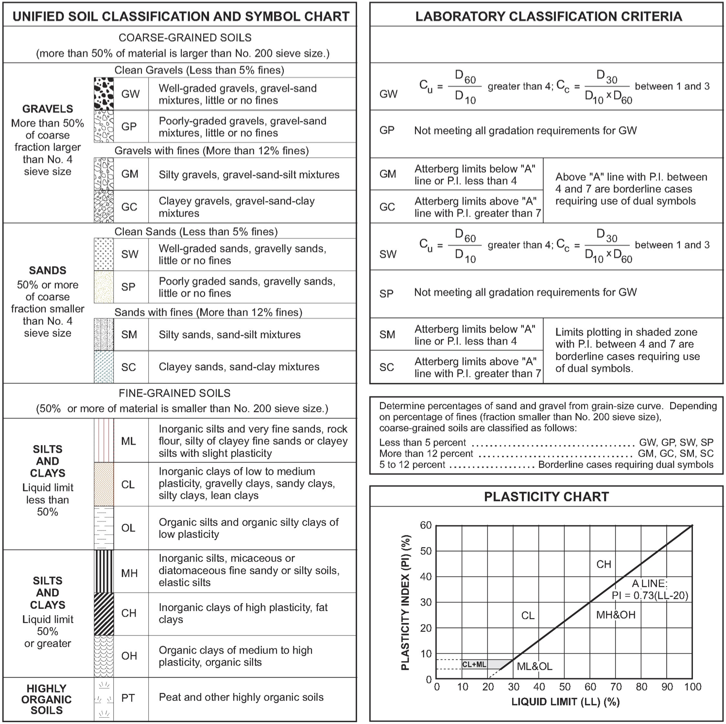
Fig. 2 Appendix: Unified Soil Classification System, USCS (adopted from the California Department of Transportation, Caltrans).

Table 6 Appendix: Unified Soil Classification System (USCS)

Soil Type	USCS Symbol	Long Description	Short Description
COARSE-GRAINED SOILS (COHESIONLESS) (more than 50% of material is larger than No. 200 sieve size)
GRAVELS More than 50% of coarse fraction larger than No. 4 sieve size	Clean Gravels (Less than 5% fines)
	GW	Well-graded gravels, gravel-sand mixtures, little or no fines	Gravel (WG)
	GP	Poorly-graded gravels, gravel-sand mixtures, little or no fines	Gravel (PG)
	Gravels with Fines (More than 12% fines)
	GM	Silty gravels, gravel-sand-silt mixtures	Silty gravel
	GC	Clayey gravels, gravel-sand-clay mixtures	Clayey gravel
	Mixed Gravels
	GW-GM	Well-graded gravels, gravel-sand mixtures, with fines	Gravel (WG, w/ fines)
	GP-GM	Poorly-graded gravels, gravel-sand mixtures, with fines	Gravel (PG, w/ fines)
SANDS 50% or more of coarse fraction smaller than No. 4 sieve size	Clean Sands (Less than 5% fines)
	SW	Well-graded sands, gravelly sands, little or no fines	Sand (WG)
	SP	Poorly-graded sands, gravelly sands, little or no fines	Sand (PG)
	Sands with Fines (More than 12% fines)
	SM	Silty sands, sand-silt mixtures	Silty sand
	SC	Clayey sands, sand-clay mixtures	Clayey sand
	Mixed Sands
	SW-SM	Well-graded sands, gravelly sands, with silt	Sand (WG, w/ silt)
	SW-SC	Well-graded sands, gravelly sands, with clay	Sand (WG, w/ clay)
	SP-SM	Poorly-graded sands, gravelly sands, with silt	Sand (PG, w/ silt)
	SP-SC	Poorly-graded sands, gravelly sands, with clay	Sand (PG, w/ clay)
FINE-GRAINED SOILS (COHESIVE) (50% or more of material is smaller than No. 200 sieve size)
SILTS AND CLAYS Liquid limit less than 50%	ML	Inorganic silts and very fine sands, rock flour, silty of clayey fine sands or clayey silts with slight plasticity	Sandy/Clayey Silt (LP)
	CL	Inorganic clays of low to medium plasticity, gravelly clays, sandy clays, silty clays, lean clays	Clay (LP)
	OL	Organic silts and organic silty clays of low plasticity	Organic silt/clay (LP)
	CL-ML		Silty Clay (LP)
	SM-ML		Sandy/Clayey Silt (LP)
SILTS AND CLAYS Liquid limit 50% or greater	MH	Inorganic silts, micaceous or diatomaceous fine sandy or silty soils, elastic silts	Sandy/Clayey Silt (HP)
	CH	Inorganic clays of high plasticity, fat clays	Clay (HP)
	OH	Organic clays of medium to high plasticity, organic silts	Organic silt/clay (HP)
	OL-OH
	CL-CH
HIGHLY ORGANIC SOILS	PT	Peat and other highly organic soils	Peat
ROCKS (not in USCS)
	ROCK		Rock

The USCS table is stored in and can be retrieved from the uscs_dict dictionary. An example is shown in Listing 1.

Listing 1 USCS table in edafos

# Import the `uscs_dict` dictionary
In [1]: from edafos.data import uscs_dict

# Query the `uscs_dict` dictionary
In [2]: uscs_dict['GP']['long_desc']
Out[2]: 'Poorly-graded gravels, gravel-sand mixtures, little or no fines'

In [3]: uscs_dict['GP']['soil_type']
Out[3]: 'cohesionless'