5. Presentation of Nominal Resistance Methods

Several pile capacity methods were used to compare calculated and predicted pile capacities. A brief overview of these methods is presented in this chapter. In order to allow for batch processing, the capacity methods were programmed in Python.

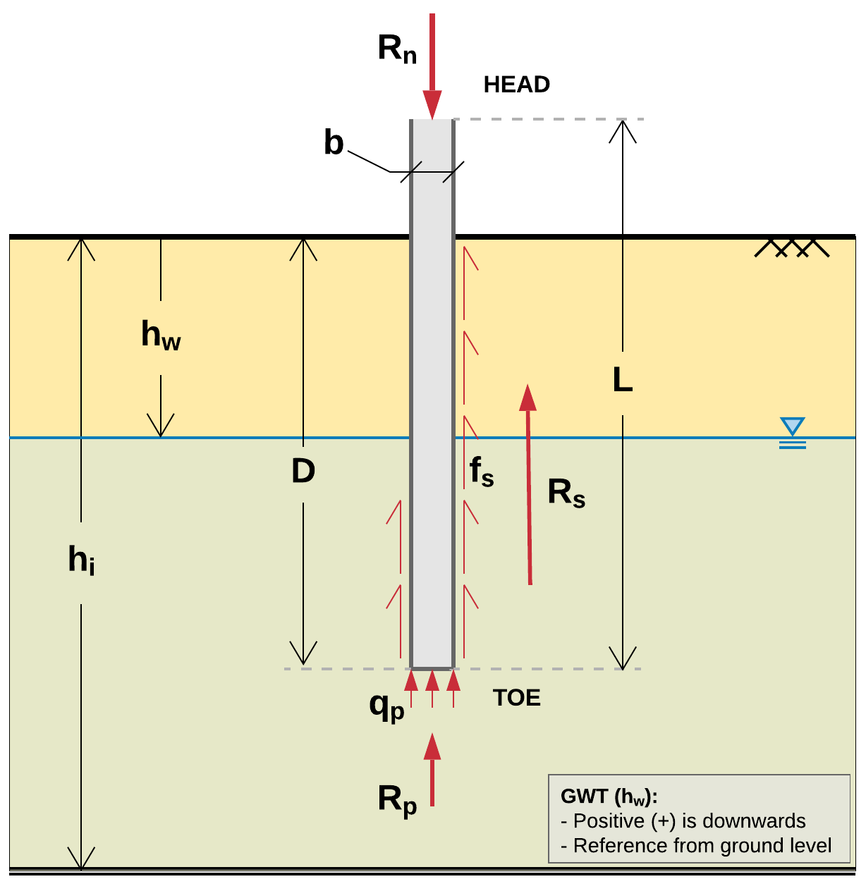
Fig. 5.1 Typical profile view with embedded pile and associated symbols

The ultimate bearing capacity, \(R_n\) (aka nominal resistance), of driven piles is typically given by nominally adding the shaft and toe resistances (Eq. 5.1).

(5.1)\[R_n = R_s + R_p = \sum f_s A_s + q_p A_p\]

where:

\(R_s\)

Shaft resistance

\(f_s\)

Unit shaft resistance, adhesion

\(A_s\)

Shaft surface area

\(R_p\)

Toe resistance

\(q_p\)

Unit toe resistance

\(A_p\)

Toe cross sectional area

For open-ended piles, soil plugging must be taken into account. In the case where a pile is plugged, capacity is calculated with Eq. 5.1 using the external side resistance and the toe resistance from the full width of the toe. However, when an open-ended pile cores the soil stratum while driving, the pile is modelled as unplugged or partially plugged and Eq. 5.1 is adjusted to account for internal and external side resistance as well as toe resistance from the pile’s annulus cross-sectional area. FHWA advises, following Paikowsky and Whitman (1990) recommendations, that static resistance of an open-ended pipe pile be calculated from the lesser of Eq. 5.2 for plugged conditions and Eq. 5.3 for unplugged conditions (Hannigan et al., 2016a).

(5.2)\[R_n = \sum f_{so} A_{so} + q_{p} A_{pp}\]

(5.3)\[R_n = \sum f_{so} A_{so} + \sum f_{si} A_{si} + q_{p} A_{p} - W_p\]

where:

\(f_{so}\)

exterior unit shaft resistance

\(A_{so}\)

exterior surface area

\(f_{si}\)

interior unit shaft resistance

\(A_{si}\)

interior surface area

\(A_{pp}\)

cross sectional area of pile and soil plug at pile toe

\(W_p\)

weight of soil plug

5.1. Nordlund Method for Cohesionless Soils

The Nordlund method (Nordlund, 1963), is recommended by FHWA (Hannigan et al., 2016a) for accurate determination of driven pile capacity in cohesionless soils. This method is semi-empirical and heavily reliant on determination of the soil friction angle, \(\phi\). Nordlund (Nordlund, 1963; Nordlund, 1979) developed his method of calculating bearing capacity of piles in cohesionless soils from as few as 41 load tests from eight different test sites. Although the method was developed for piles smaller than 18 inches in diameter, it is still the most widely used method in State DOTs for the design of all driven piles, including LDOEPs (NCHRP 2015).

For uniform (non-tapered) piles, side resistance by the Nordlund method is calculated using Eq. 5.4 and toe resistance is calculated using Eq. 5.5. The method uses corrected SPT N-values (or, preferably, lab-produced strength parameters) to determine the soil friction angle for each soil layer and uses a series of published tables and charts to assume correlations for the coefficient of lateral earth pressure and the soil-pile friction angle. These values are used along with the effective overburden pressure, to determine the side resistance for each defined layer. Pile tip bearing capacity factors are also correlated from the soil friction angle using charts. Upper limits are placed upon skin friction and pile tip resistance, \(R_p\), in order to limit the magnitude of the computed unit skin and tip resistance and calculate a safer ultimate pile capacity.

(5.4)\[R_s = \sum K_d \, C_F \, \sigma'_d \, \sin(\delta) \, C_d \, \Delta d\]

(5.5)\[R_p = \alpha_t \, N'_q \, A_p \, \sigma'_p\]

where:

\(K_d\)

coefficient of lateral earth pressure at depth \(d\)

\(C_F\)

correction factor for \(K_d\) when \(\delta \neq \phi\)

\(\sigma'_d\)

vertical effective stress at the center of depth increment \(d\)

\(\delta\)

friction angle between pile and soil

\(C_d\)

pile perimeter at depth \(d\)

\(\Delta_d\)

length of pile segment

\(\alpha_t\)

dimensionless factor (dependent on pile depth width relationship)

\(N'_q\)

bearing capacity factor

\(\sigma'_p\)

vertical effective stress at pile toe

5.2. Tomlinson Method for Cohesive Soils

The FHWA Report on the Design and Construction of Driven Pile Foundations (Hannigan et al., 2016a; Hannigan et al., 2016b) recommends that for pile diameters less than 18 inches, nominal resistance be calculated using the \(\alpha\)-method (Tomlinson, 1980) for cohesive soils. Similar to the Nordlund method, it is the most widely used method in State DOTs for the design of all driven piles in cohesive soils, including LDOEPs (NCHRP 2015).

The \(\alpha\)-method, is an empirical total stress calculation method that uses the undrained shear strength of soil to find ultimate pile capacity. The unit skin resistance is shown by Tomlinson to be equal to the adhesion of soil to the pile, which is given by an “alpha” (\(\alpha\)) factor determined by soil and pile properties using original tables and the undrained shear strength, \(s_u\), with \(f_s = \alpha s_u\). Values of \(\alpha\) are inversely proportional to the undrained shear strength of the soil and are always less than 1, due to the adhesion between the pile and soil always being less than the cohesion within the soil.

In cohesive layers, side and toe resistances calculated by the \(\alpha\)-method are based on Eq. 5.6 & Eq. 5.7. When dealing with mixed soil profiles, Tomlinson provides adjustment factors to account for drag-down of weaker soils into stiffer layers, a phenomenon that occurs during pile driving and reduces the side resistance. These factors were accounted for in our calculations.

(5.6)\[R_s = \sum f_s A_s = \sum C_\alpha A_s = \sum \alpha \, s_u \, A_s\]

(5.7)\[R_p = q_p A_p = N_c s_u A_p\]

where:

\(C_\alpha\)

adhesion

\(\alpha\)

adhesion factor

\(s_u\)

undrained shear strength

\(A_s\)

shaft surface area

\(N_c\)

bearing capacity factor

Note

For plugged and unplugged analyses, Eq. 5.4 through Eq. 5.7 must be adjusted according to Eq. 5.2 & Eq. 5.3.

5.3. United States Army Corps of Engineers (USACE) Method

For side resistance in cohesionless soils, USACE specifies that skin friction increases linearly down to a critical depth, \(D_c\), and remains constant below that depth. The critical depth, \(D_c\), is a function of pile diameter, \(b\), such that \(D_c = 10b\) for loose sands, \(D_c = 15b\) for medium-dense sands and \(D_c = 20b\) for dense sands. Side resistance can then be calculated according to Eq. 8.

(5.8)\[R_s = \sum f_s A_s = \sum K \, \sigma'_v \, \tan \delta \, A_s\]

where:

\(K\)

lateral earth pressure coefficient

\(\sigma'_v\)

vertical effective overburden pressure (\(\sigma'_v = \gamma' D\) when \(D<D_c\) or \(\sigma'_v = \gamma' D_c\) when \(D \geq D_c\))

\(\delta\)

angle of friction between pile and soil (from USACE, 1991)

\(\gamma'\)

effective unit weight of soil

\(D\)

depth along the pile

For toe resistance in cohesionless soils, the same critical depth relationship as for skin friction can be used. Toe resistance can then be calculated according to Eq. 5.9.

(5.9)\[R_p = q_p A_p = \sigma'_v \, N_q \, A_p\]

where:

\(\sigma'_v\)

vertical effective overburden pressure (\(\sigma'_v = \gamma' D\) when \(D<D_c\) or \(\sigma'_v = \gamma' D_c\) when \(D \geq D_c\))

\(N'_q\)

bearing capacity factor (from Terzaghi and Peck, 1967)

For side resistance in cohesive soils, the USACE method is largely similar to the \(\alpha\)-method in that resistance is due to the adhesion of the cohesive material to the side of the pile and is calculated according to Eq. 5.10.

(5.10)\[R_s = \sum f_s A_s = \sum c_a \, A_s = \sum \alpha \, s_u \, A_s\]

where:

\(C_\alpha\)

adhesion between pile and cohesive soil

\(\alpha\)

adhesion factor (from USACE, 1991)

Toe resistance in cohesive soils is calculated by USACE according to Eq. 5.11.

(5.11)\[R_p = q_p A_p = 9 \, s_u \, A_p\]

where:

\(s_u\)

undrained shear strength at pile toe, normally the average over a depth of two pile diameters below the toe

Note

For plugged and unplugged analyses, Eq. 5.8 through Eq. 5.11 must be adjusted according to Eq. 5.2 & Eq. 5.3.

5.4. Revised Lambda Method

The Lambda method has gone through several revisions since it was first introduced. Focht and Vijayvergiya (1972) proposed that side resistance be calculated using Eq. 5.12.

(5.12)\[R_s = \sum f_s A_s = \sum \lambda \, (\bar{\sigma'} + 2 \bar{s_u}) \, A_s\]

where:

\(\lambda\)

pile penetration coefficient

\(\bar{\sigma'}\)

average vertical effective stress between the ground surface and the pile toe

\(\bar{s_u}\)

average undrained shear strength

Kraft et al. (1981) revised the pile penetration coefficient, \(\lambda\), proposing formulas for normally consolidated soils (Eq. 5.13) and overconsolidated soils (Eq. 5.14). When information on consolidation was missing or was unreliable, cohesive soils were assumed to be over-consolidated if \(s_u/\sigma\) was equal to or larger than 0.1.

(5.13)\[\lambda = 0.178 - 0.016 \ln \pi_3\]

(5.14)\[\lambda = 0.232 - 0.032 \ln \pi_3\]

where:

\(\pi_3\)

\(\dfrac{\pi b f_{s.max}D^2 }{AEU}\)

\(b\)

pile diameter

\(f_{s.max}\)

peak unit skin friction

\(D\)

embedded pile length

\(A\)

cross-sectional area

\(E\)

modulus of elasticity

\(U\)

pile displacement needed to develop side shear (normally 0.1 inch)

5.5. American Petroleum Institute (API) Method

The API design method is widely regarded as the best method for the design of LDOEPs due to the Institute’s long history in the design of offshore platforms. It was presented in the “Recommended Practice” Report RP-2A in 1986 and was revised in 1987 and 1993. Side resistance in cohesionless soils can be calculated using Eq. 5.15.

(5.15)\[R_s = \sum f_s A_s = \sum K \, \bar{\sigma'} \, \tan \delta \, A_s\]

where:

\(K\)

coefficient of lateral earth

\(\bar{\sigma'}\)

average vertical effective stress

\(\delta\)

angle of friction between pile and soil (API RP-2A, 1993)

Table 5.1 offers recommended values for the coefficient of lateral earth, \(K\).

Table 5.1 Values for coefficient of lateral earth, \(K\)

Condition	K
unplugged, open-ended pipe piles (tens & comp)	0.8
full-displacement piles	1.0

Table 5.2 offers guidelines for \(\delta\), the friction angle between the soil and the pile wall as well as limiting unit friction, \(f_s\).

Table 5.2 API Guidelines for Side Friction in Siliceous Soil

Soil	\(\delta\) , degrees	Limiting, \(f_s\)
		kips/ft2 | kPa
Very loose to medium, sand to silt	15	1.0	47.8
Loose to dense, sand to silt	20	1.4	67.0
Medium to dense, sand to sand-silt	25	1.7	81.4
Dense to very dense, sand to sand-silt	30	2.0	95.8
Dense to very dense, gravel to sand	35	2.4	114.9

Toe resistance in cohesionless soils is given by Eq. 5.16.

(5.16)\[R_p = q_p A_p = \sigma' N_q \, A_p\]

where:

\(\sigma'\)

effective stress at pile toe

\(N'_q\)

bearing capacity factor

Neither unit shaft resistance, \(f_s\), nor unit toe resistance, \(q_p\), increase linearly without limit. API RP-2A limiting unit shaft and toe resistance values based on soil consistency, from very loose sand/silt to very dense sand/gravel.

Table 5.3 offers guidelines for \(N_q\), bearing capacity factor as well as limiting, \(q_p\).

Table 5.3 API Guidelines for Toe Resistance in Siliceous Soil

Soil	\(N_q\)	Limiting, \(q_p\)
		kips/ft2 | MPa
Very loose to medium, sand to silt	8	40	1.9
Loose to dense, sand to silt	12	60	2.9
Medium to dense, sand to sand-silt	20	100	4.8
Dense to very dense, sand to sand-silt	40	200	9.6
Dense to very dense, gravel to sand	50	250	12.0

The general equation for shaft resistance in cohesive soils according to the revised API method is presented in Eq. 5.17.

(5.17)\[R_s = \sum f_s A_s = \sum \alpha s_u \, A_s\]

(5.18)\[\begin{split}\alpha = \begin{cases} 0.5\psi^{-0.5} & \textrm{if} \quad \psi \leq 1.0 \\ 0.5\psi^{-0.25} & \textrm{if} \quad \psi > 1.0 \end{cases} \quad \leq 1.0\end{split}\]

where:

\(\alpha\)

adhesion coefficient governed by Eq. 5.18 where \(\psi = s_u/\bar{\sigma'}\)

\(\bar{\sigma'}\)

average vertical effective stress

Finally, toe resistance in cohesive soils is given by Eq. 5.19, the same way as for the USACE method.

(5.19)\[R_p = q_p A_p = 9 \, s_u \, A_p\]

Important

• Toe resistance must always be checked against \(R_p = q_p A_{pp}\) where \(A_{pp}\) is the cross sectional area of soil plug in open end pipe or H-piles at pile toe.

• Undrained shear strength at the toe of the pile, \(s_u\), is usually taken as the average over a distance of two diameters below the tip of the pile.

Note

For plugged and unplugged analyses, Eq. 5.15 through Eq. 5.19 must be adjusted according to Eq. 5.2 & Eq. 5.3.

In order to interpret Table 5.2 and Table 5.3 algorithmically, the correlation in Table 5.4 was employed in batch calculations.

Table 5.4 SPT-N corrected Correlations

Density	\(N_{cor}\) (bpf)	\(\phi\) (deg)
Very loose	0 - 4	< 28
Loose	5 - 10	28 - 30
Medium dense	11 - 30	30 - 36
Dense	31 - 50	36 - 41
Very Dense	over 50	> 41

In which case Table 5.2, Table 5.3 and Table 5.4 can be consolidated as in Table 5.5.

Table 5.5 API Guidelines for Shaft and Toe Resistance in Siliceous Soil with SPT-N values

Soil	\(N_{cor}\) (bpf)	\(\delta\) (deg)	\(f_{s.lim}\) (ksf)	\(N_q\)	\(q_{p.lim}\) (ksf)
Very loose to medium, sand to silt	0 - 4	15	1.0	8	40
Loose to dense, sand to silt	5 - 10	20	1.4	12	60
Medium to dense, sand to sand-silt	11 - 30	25	1.7	20	100
Dense to very dense, sand to sand-silt	31 - 50	30	2.0	40	200
Dense to very dense, gravel to sand	over 50	35	2.4	50	250

5.6. Olson 90 Method

The Olson 90 method is for cohesionless soils only. It was created from a database of 31 load tests on steel pipe piles. Olson 90 is similar to the Revised API method with two main differences. First, the coefficient of lateral earth, \(K\), is calculated rather than taken from Table 5.1. In Olson 90, \(K\) is given by Eq. 5.20.

(5.20)\[\begin{split}K = \begin{cases} 0.16 + 0.015 \, N_{cor} & \textrm{non-displacement piles}\\ 0.70 + 0.015 \, N_{cor} & \textrm{full displacement piles} \end{cases}\end{split}\]

Olson 90 provides revised guidelines for shaft and tow resistances and they are summarized in Table 5.6.

Table 5.6 Olson 90 guidelines for Shaft and Toe Resistance

Soil	\(N_{cor}\) (bpf)	\(\delta\) (deg)	\(f_{s.lim}\) (ksf)	\(N_q\)	\(q_{p.lim}\) (ksf)
Gravel	0 - 4	[20]	[1.4]	[12]	[60]
	5 - 10	[25]	[1.7]	[20]	[100]
	11 - 30	[30]	[2.0]	[40]	[200]
	over 30	[35]	[2.4]	[60]	[250]
Sand / Gravel	0 - 4	[20]	[1.4]	[12]	[60]
	5 - 10	[25]	[1.7]	[20]	[100]
	11 - 30	[30]	[2.0]	[40]	[200]
	over 30	[35]	[2.4]	[60]	[250]
Sand	0 - 4	[20]	[1.0]	[50]	[40]
	5 - 10	30	1.1	120	120
	11 - 30	35	1.9	120	190
	31 - 50	40	2.6	120	190
	51 - 100	40	3.7	130	200
	over 100	40	3.8	220	530
Sand / Silt	0 - 4	10	[1.0]	[10]	[10]
	5 - 10	10	[1.0]	[20]	[40]
	11 - 30	15	[1.4]	50	110
	31 - 50	20	2.0	100	160
	51 - 100	[30]	[2.0]	[100]	[200]
	101 - 200	[34]	[20]	[100]	[200]
	over 200	40	20	[100]	[200]
Silt	0 - 4	[10]	[1.0]	[10]	[40]
	5 - 10	15	[1.0]	[10]	[40]
	11 - 30	20	[1.4]	[10]	[40]
	31 - 50	20	[1.4]	[12]	[60]
	over 50	[25]	[1.4]	[12]	[60]

Note

For Table 5.6

• Must not interpolate. In using values in Table 5.6, use the line corresponding to N = 4 for any layer with N less than or equal to 4, the line corresponding to 10 for N = 5 - 10, and so on.

• Number in brackets were extrapolated, no supporting data.